1 Introduction
This technical note describes a series of tests performed with a Cassandra-based APDB implementation on the Google Cloud Platform (GCP). A previous round of APDB tests with Apache Cassandra performed with a three-node cluster at NCSA (DMTN-156) showed promising results, but it was not possible to evaluate scaling behavior from those tests. A subsequent series of tests was necessary at larger scale, and a plan for those tests was outlined in DMTN-162. Actual testing was performed using GCP resources which allowed us to chose the optimal configuration for each test. Cluster setup and all tests are described in more detail in JIRA tickets under the DM-27785 epic.
2 Cluster Configuration
GCP was used to run both the Cassandra server cluster and the client software. On
the client side we ran 189 processes executing the ap_proto application
which did not require significant resources. To avoid over-subscribing CPU
resources we were allocating one vCPU per process; the cluster that was used to
run the client software was comprised of 6 nodes, each of e2-custom type, with 32
vCPUs and 16GB RAM. The nodes were using the lsst-w-2020-49 image with LSST
software pre-installed. Client process execution was orchestrated using the MPI
mechanism, similar to how it was done at NCSA.
The Cassandra cluster is more resource-demanding; from our previous tests at NCSA it was clear that fast SSD storage is critical for performance and Cassandra in general needs abundant RAM, though too much RAM can cause issues with garbage collection. For these reasons the configuration for a single node in Cassandra cluster was selected as:
- n2-custom VM type
- 32 vCPUs
- 64 GB RAM
- locally attached SSD storage, 4 or 8 partitions, 375 GB each
- Ubuntu-based image which is recommended for optimized nVME drivers
GCP locally attached SSDs are non-persistent (scratch) and they are re-created on each VM reboot, so special care is needed in planning the tests. Cassandra cluster size was varied between 3 and 12 nodes to evaluate scaling behavior.
The Cassandra configuration needed the usual update for some of its parameters, a copy
of the configuration files
is archived in the l1dbproto package for future reference.
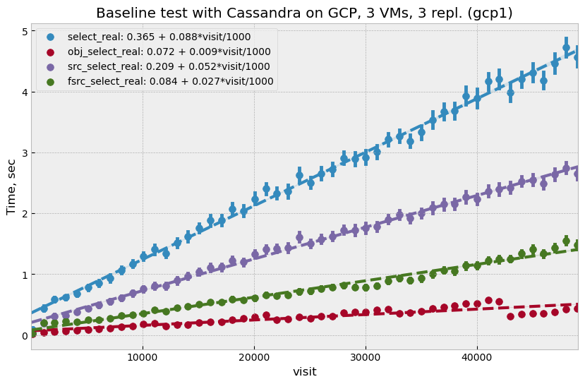
3 Three-node Setup
The very first test (DM-28136) done with the new platform was a
repeat of the setup used for on-prem APDB tests at NCSA. The goals of this test were to
verify that things worked as expected, that performance was not worse than what
was observed in the NCSA tests, and to set a baseline for scalability testing. For
this and all following tests we used a replication factor of 3 and consistency level
QUORUM for both reading and writing.
In total, 50k visits were generated for this test. Performance looked similar to what was observed at NCSA with same linear growth of read time with the number of visits. Actual read time was improved slightly compared to NCSA; at 50k visits total select time for all three tables was below 5 seconds, while NCSA performance was closer to 7 seconds for the same 50k visits.
4 Six-node Setup
The next test (DM-28154) was to check how performance improved with increased cluster size by doubling the number of nodes. Ideally, Cassandra performance should scale linearly with the number of nodes and read time should reduce by 50%.
On the first iteration, 75k visits were generated but performance did not improve as expected; total
read time at 50k visits was around 3.1 sec which was about a 35% improvement
compared to the three-node case. Profiling showed that a significant fraction of time
on the client side was spent converting the data into afw.Table format, which
was used as a return data type for APDB API in these tests.
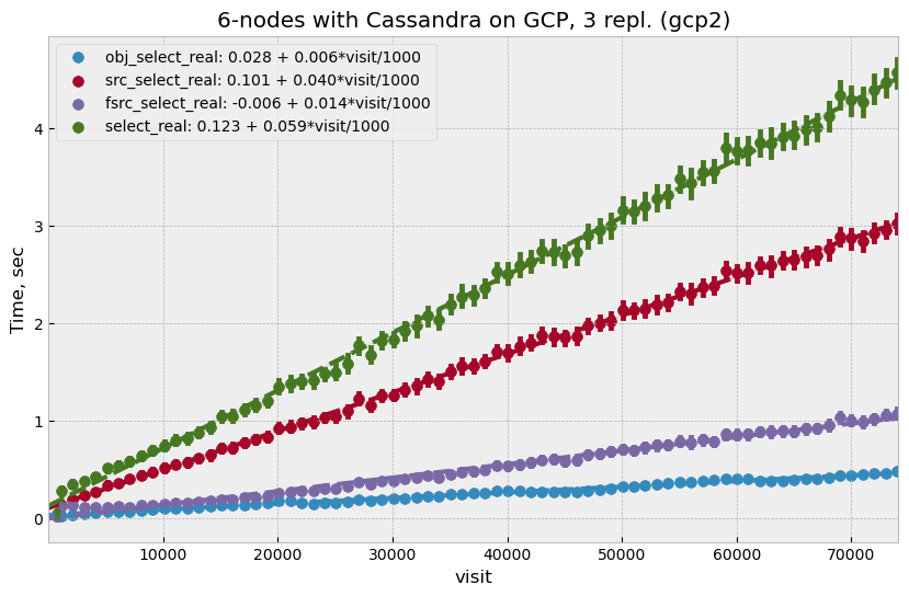
As the AP pipeline has already decided to switch to pandas instead of afw.Table
for its internal presentation, we decided to switch to pandas as well, and
repeated the six-node test using that data format. There were 100k visits generated
in the second iteration of this test, with pandas total read time reduced to
1.67 seconds at 50k (and 3.26 sec at 100k visits), and CPU time on the client side
reduced dramatically. We did not repeat the three-node test with pandas;
instead we proceeded to a larger scale test.
5 Twelve-node Setup
The next test (DM-28172) increased the scale of the Cassandra cluster to 12 nodes. The goal for this test was to further observe scaling behavior but also to extend the test beyond 12 months of visits to see how performance behaves when history size for DiaSources and DiaForcedSources stops growing. For this test we increased SSD storage size to 3TB (8 partitions) on each node. In total there were 450k visits generated in this test.
5.1 Scaling Behavior
Compared to the previous six-node test, performance improved significantly and total read time dropped to 1.65 sec at 100k visits, which is about 50% improvement compared to the six-node setup.
Figure 1 shows a summary of scaling behavior for all
of the above tests. After fixing excessive CPU usage by the afw.Table conversion code,
scaling behavior practically matches the ideal 1/N curve.
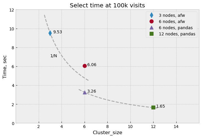
Figure 1 Summary of reading performance as a function of number of nodes. Performance
is given as a total read time at 100k visits, with three-node and six-node
afw.Table cases extrapolated to 100k. Curves represent ideal 1/N
scaling behavior.
5.2 Twelve-month Plateau
As seen on all previous plots, select time grows linearly with the number
of DiaSources and DiaForcedSources. Those numbers are determined by the size of
the history read from database which is set to 12 months. We expect the numbers
to plateau after 12 months and for read time to stabilize. To
demonstrate this, we generated 450k of visits, which corresponds approximately to
18 months of calendar time. ap_proto generates 800 visits per night, which translates
into 288k visits for twelve 30-night “months”.
Figure 2 shows select time behavior for the whole range of generated visits. It is clear that after 300k visits, select time stabilizes at the level of 4.5 seconds per visit. The sawtooth-like fluctuations after 300k visits are related to the time partitioning scale, which is 30 days in this case. This plot shows select time which is averaged over multiple of visits; there are of course significant visit-to-visit fluctuations. Figure 3 shows a scatter plot of select and insert times for individual visits without averaging; visit-to-visit fluctuations are clearly visible but they stay in reasonable range.
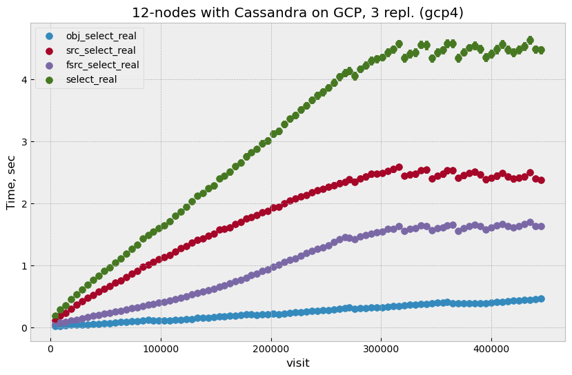
Figure 2 Time to read as a function of visit for all three tables, select_real is
a sum of three other values. Total time plateaus after approximately 300k
visits, small fluctuations are due to granularity of time partitioning.
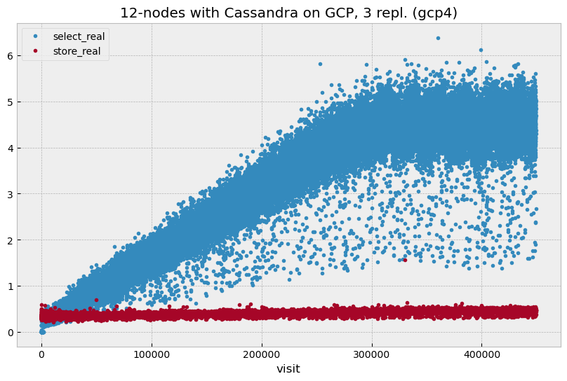
Figure 3 Scatter plot for select and insert time showing times for individual visits. Blue markers correspond to averaged green markers on the above plot.
6 Partitioning Options
For all of the above test we used identical partitioning options:
- MQ3C(10) spatial partitioning
- 30 day time partitioning for DiaSource and DiaForcedSource
- time partition is not using Cassandra partitioning but separate per-partition tables instead
Optimal partition sizes should provide a balance between the number of partitions queried and the size of the data returned. Smaller partition sizes will reduce overhead in the size of the returned data but will increase the number of queries needed to select the data. Time partitioning is implemented using separate per-month tables; this is done to simplify management of the data beyond 12 months. Older data that will not be queried after 12 months can be moved to slower storage or archived to save on SSD storage cost; that process will be easier to implement with the data in separate tables.
Part of the epic was devoted to testing possible options for partitioning that could potentially improve performance. These are described below.
6.1 Partitioning Granularity
Reducing the partition granularity decreases the number of partitions, and consequently the number of separate queries that need to be executed to get the same data; this could have an impact on server performance. To check that we reduced the size of the timing partitions from 30 days to 60 days and re-ran the test (DM-28467). There was no visible change in timing for select queries on the client side, while server side monitoring showed some moderate improvement in resource usage. Given that overall performance does not improve, it makes sense to keep the granularity at 1 month to limit the overhead in the size of the data returned to clients.
6.2 Native Time Partitioning
While using separate-table partitioning for the time dimension has management benefits, it could also have some performance impact. To quantify this we performed a test where the separate-table partitioning mechanism was replaced with native Cassandra partitioning (DM-28522).
As before, no significant difference in select time was observed with this change.
6.3 Query Format
Cassandra query language is limited in what it can do but there is some freedom in how queries can be formulated to select data from multiple partitions:
- execute a single query specifying all partitions in
IN()expression, e.g.SELECT ... WHERE partition IN (...) - execute multiple queries, one query per partition, e.g.
SELECT ... WHERE
partition = ...
The difference between these two options is where the merging of the results happens; in the former case the merge is done server side by the coordinator node, in the latter case the client is responsible for merging.
We tested both options for querying time partitions (when time was natively partitioned) and did not find a significant difference in performance between them. While queries cover only 13 time partitions, for spatial indexing the number of partitions per visit is higher. When we tried an extreme case with individual queries for each temporal and spatial partition then total number of separate queries grew to more than 200. Client side performance in this case was significantly worse, with the client spending significant CPU time on the processing of multiple results.
7 Packed Data
The schema of the Cassandra tables follows the definition outlined in the DPDD. The DiaObject and DiaSource tables are very wide and have a large number of columns. Most of these columns are never used by Cassandra; there are no indices defined for them and queries do not use them. Management overhead for the schema could be reduced if the bulk of that data were to be stored in some opaque form. Packing most columns in a BLOB-like structure on the client side could have some benefits but may also have some serious drawbacks:
- server-side operations may become faster if the server does not need to care about individual columns
- potential schema change management may be simplified
- if packing format is dynamic, it needs extra space for column mapping
- significantly more work needed on client side to pack/unpack the data
A simple test was done to check how this might work (DM-28820). For serialization of records we used CBOR which is a compact binary JSON-like format. CBOR structure is dynamic and needs to pack all column names with the data, thus inflating the size of the BLOB. Cassandra uses compression for the data saved on disk which could offset some of that inflated size.
The results from this test showed that performance was slower in this case, caused by significantly higher client side CPU usage spent on query result conversion. Attempts to optimize the conversion were only partially successful; improvements may be possible in general but would require doing much of the conversion in C++.
Disk usage in Cassandra was increased by factor of two in this scenario, even if the compression ratio for the data was increased. Given all these observation, our simple approach clearly does not result in improvement. It may still be possible to achieve some gains with packing, but it would require significant effort to use a fixed schema client side and optimize the conversion performance.
7.1 Pandas Performance
The results of this test also show a potential for improvement. Converting
query results to pandas format requires significant client side effort.
The main reason for this is a mismatch between the data representation used by
the Cassandra client and that used by pandas. The Cassandra client produces result data as a
sequence of tuples which is a close match to its wire-level protocol. pandas on
the other hand keeps the data in memory as a set of two-dimensional arrays.
Transformation of these tuples to arrays involves a lot of iterations that all happen
at the Python level. If further improvements for conversion are necessary one could
think of either replacing pandas with a format that better matches
the Cassandra representation or rewriting the expensive parts of the conversion in C++.
8 High Availability
One unplanned test happened by accident but allowed us to check how well the high availability feature of Cassandra performs (DM-28522). One of the eight Cassandra nodes was misconfigured and its server became unavailable for several hours. Despite that, the cluster continued functioning normally without much of impact on performance. Both read and write latencies stayed at the same level, though obviously timeouts did happen when some clients that connected to that particular instance had to wait for a response before the cluster declared the node to be dead.
After the instance was reconfigured and re-joined the cluster all operations continued and monitoring showed that data recovery on the temporary unavailable node worked as expected. This incident shows that Cassandra can function without service degradation when one replica becomes inaccessible. Cassandra has a flexible consistency model which can be tuned for particular operation models.
9 Other observations
9.1 High CPU Usage
Monitoring the Cassandra cluster showed that occasionally one or two servers could start showing high CPU usage compared to all other servers. It did not seem to affect overall performance very much; a noticeable effect was seen only on write latency which still stayed reasonably low. It seems that the issue can be mitigated by restarting that particular instance. After the restart CPU usage returns to normal. This may be related to how the cluster is initialized, as it was only seen when the cluster was re-initialized from scratch. We tried to get some advice from the Cassandra developers on this issue, but none of the suggestion we received helped to understand the cause.
9.2 What Was Not Tested
The tests with the AP prototype represent just a basic part of the AP pipeline operation. Some more complicated options are not implemented in the prototype, in particular:
- Day-time re-association of DiaSources to SSObjects is not implemented and was not tested. Due to Cassandra’s architecture update operations are not trivial and may have some impact on later read requests. It may be possible to avoid this completely by splitting the table schema, and it clearly deserves a separate test.
- Possible concurrent access to APDB data by other clients was not tested. At this point it is not clear what these other clients could be.
- Variability of DiaSources density.
ap_protocurrently uses a uniform distribution for DiaSources. It would be interesting to see the effect of non-uniformity on performance. - Data management aspects of the operations were not tested. Such operations would include archiving or removal of older data and cleanup of the tables. This aspect will need to be understood and tested as well.
10 Conclusion
We tested the APDB prototype against a Cassandra cluster running on GCP using different options for cluster size and for its operating parameters. A twelve-node Cassandra cluster seemed to provide performance that could be adequate for AP pipeline operation for the scale of one year and beyond. The tests also provided valuable insight into the operation of a Cassandra cluster and the potential for further client side performance improvements.